Compound Annual Growth Rate, CAGR, is your rate of return for an investment over a specific period.

Calculating CAGR by hand is a rather involved process, so below we’ll go over how you can quickly calculate CAGR in Excel.

CAGR Excel Formula

The formula for calculating CAGR in Excel is:

=(End Value/Beginning Value) ^ (1/Number of Years) – 1

The equation uses three different values:

• End value, which is the amount of money you’ll have after the period has passed.
• Beginning value, which is the amount of money you began with.
• Number of years, which is the total number of years that have passed.

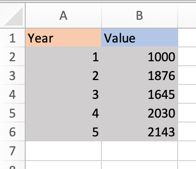
Below we’ll go over an example of how to calculate CAGR for a five years time frame in Excel using the sample data set shown below:

1. Identify the numbers you’ll use in your equation. Using the sample data set above,

• The end value is 2143 (in cell B6).
• The beginning value is 1000 (in cell B2).
• The number of years is 5 (in cell A6).

2. Input your values into the formula. 

Excel offers many shortcuts, so you can simply input the cell numbers that contain each of your values into the equation. Using the sample data set above, the equation would be

=(B6/B2) ^ (1/A6) – 1

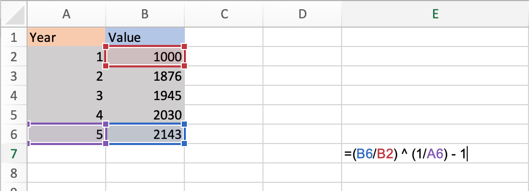
This is what it looks like in my Excel sheet:

Note that the equation changes color to correspond with the cells you’re using, so you can look back and check that your inputs are correct before running the equation.

You can also enter actual values into the formula instead of cell numbers. The equation would then look like this:

=(2143/1000) ^ (1/5) – 1

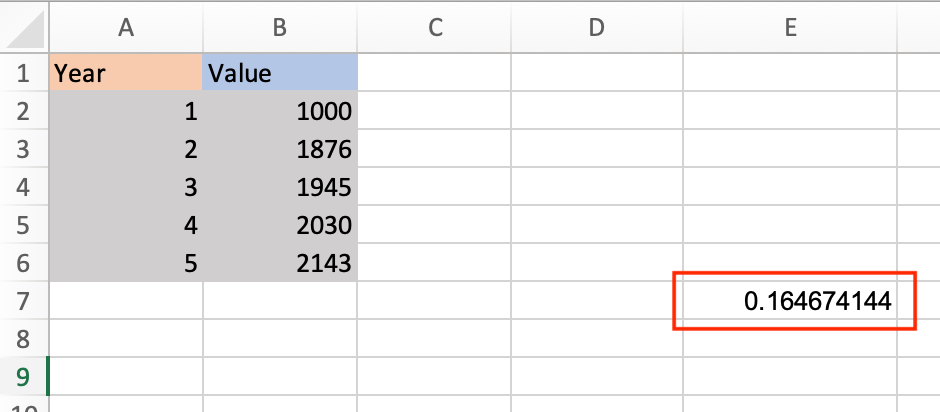
3. Once you’ve entered your values, click enter and run the equation. Your result will appear in the cell containing the equation, as shown in the image below.

CAGR Formula in Excel as a Percentage

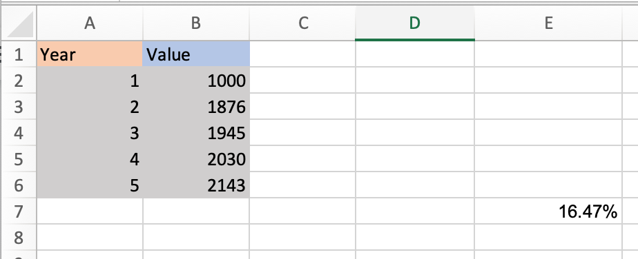
Your default result will be shown as a decimal. To view it as a percentage, right-click on the cell your result is in, select Format Cells and then Percentage in the dialogue box.

Your result will be converted to a percentage, as shown in the image below.

Now let’s go over a shortcut for calculating CAGR in Excel using the Rate function.

How To Calculate CAGR Using RATE Function

The RATE function helps you calculate the interest rate on an investment over a period of time.The formula for calculating CAGR is: 

=RATE(nper,, pv, fv)

• nper is the total number of periods in the time frame you’re measuring for. Since you’re calculating annual growth rate, this would be 12.
• pv is the present value of your investment (must always be represented as a negative)
• fv is future value.

Note that the standard RATE equation includes more variables, but you only need the above three to calculate your CAGR.

Let’s run an equation using the sample table below where nperi is 12, pv is 100, and fv is 500.

1. In your sheet, select the cell that you want to contain your CAGR. I selected cell B5.

2. Enter the RATE formula and input your numbers. Note that you always need to express your present value as a negative, or you’ll receive an error message.

This is what my formula looks like.

Note that you can also simply enter the cell numbers that your values are in. With my sample table the formula would look like this:

=RATE(A2,,-B2,C2)

3. Click enter and run your equation. Using the sample data, my CAGR is 14%.

Now you know how to quickly and easily calculate your CAGR in Excel, no hand calculations required.