

How to Highlight Duplicates in Google Sheets [Step-by-Step]
Duplicate data is the bane of spreadsheet solutions, especially at scale. Given the volume and variety of data now entered by teams, it’s possible that duplicate data in tools like Google Sheets may be relevant and necessary, or it could be a frustrating distraction from the primary purpose of spreadsheet efforts.
The potential problem raises a good question: How do you highlight duplicates in Google Sheets?
We’ve got you covered with a step-by-step look at how to highlight duplicates in Google Sheets, complete with images to make sure you’re on the right track when it comes to de-duplicating your data.
![→ Access Now: Google Sheets Templates [Free Kit]](https://no-cache.hubspot.com/cta/default/53/e7cd3f82-cab9-4017-b019-ee3fc550e0b5.png)
Highlighting Duplicate Data in Google Sheets
Google Sheets is a free, cloud-based alternative to proprietary spreadsheet programs and — no surprise, since it’s Google we’re dealing with — offers a host of great features to help streamline data entry, formatting, and calculations.
Google Sheets has all the familiar functions: File, Edit, View, Format, Data, Tools, etc. and makes it easy to quickly enter your data, add formulas for calculations, and discover key relationships. What Sheets doesn’t have, however, is an easy way to find and highlight duplicates.
While other spreadsheet tools, such as Excel, have built-in conditional formatting tools that can pinpoint duplicate data in your sheet, Google’s solution requires a little more manual effort.
Step-by-Step: How to Highlight Duplicates in Google Sheets (With Pictures)
So how do you automatically highlight duplicates in Google Sheets? While there’s no built-in tool for this purpose, you can leverage some built-in functions to highlight duplicate data.
Here’s a step-by-step guide:
Step 1: Open your spreadsheet.
Step 2: Highlight the data you want to check.
Step 3: Under “Format”, select “Conditional Formatting.”
Step 4: Select “Custom formula is.”
Step 5: Enter the custom duplicate checking formula.
Step 6: Click “Done” to see the results.
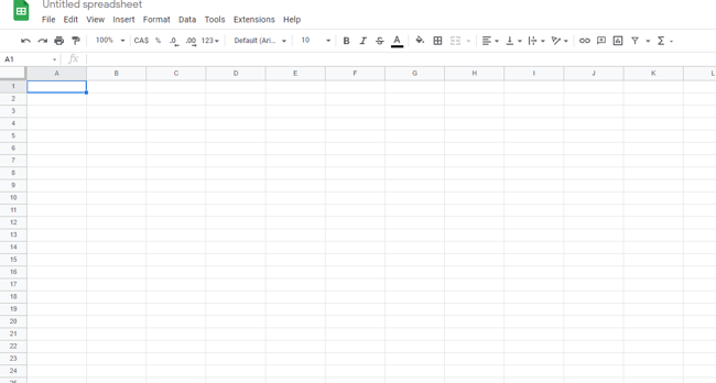
Step 1: Open your spreadsheet.
First, head to Google Sheets and open the spreadsheet you want to check for duplicate data.
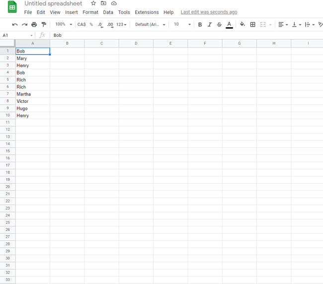
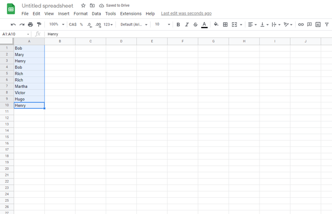
Step 2: Highlight the data you want to check.
Next, left-click and drag your cursor over the data you want to check to highlight it.
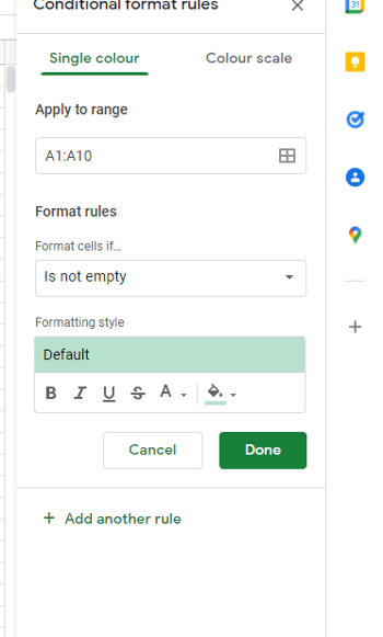
Step 3: Under “Format”, select “Conditional Formatting.”
Now, head to “Format” in the top menu row and select “Conditional Formatting”. You may get a notification that says “cell is not empty” — if so, click on it, and you should see this:
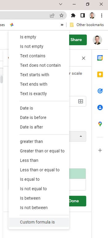
Step 4: Select “Custom formula is.”
Next, we need to create a custom formula. Under “Format cells if”, select the drop-down menu and scroll down to “Custom formula is”.
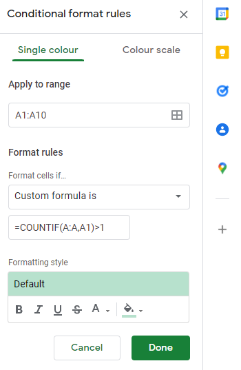
Step 5: Enter the custom duplicate checking formula.
To search for duplicate data, we need to enter the custom duplicate checking formula, which for our column of data looks like this:
=COUNTIF(A:A,A1)>1
This formula searches for any text string that appears more than once in our selected data set, and by default will highlight it in green. If you prefer a different color, click on the small paint pot icon in the formatting style bar and select the color you prefer.
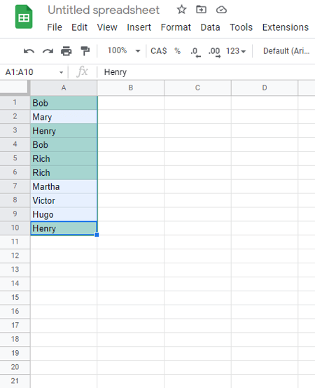
Step 6: Click “Done” to see the results.
And voilà — we’ve highlighted the duplicate data in Google Sheets.
How to Highlight Duplicates in Multiple Rows and Columns
If you’ve got a larger data set to check, it’s also possible to highlight data duplicates in multiple columns or rows.
This starts the same way as the duplicate checking process above — the only difference is that you change the data range to include all the cells you want to compare.
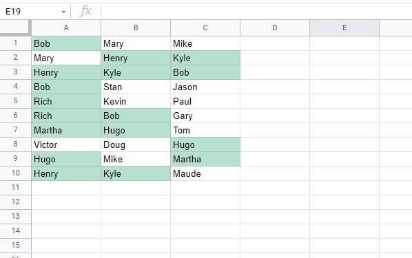
In practice, this means entering an expanded data range in the Conditional format rules menu and the custom format box. Let’s use the example above as a starting point, but instead of just searching column A for duplicates, we’re going to search across three columns: A, B, and C, and also across rows 1-10.
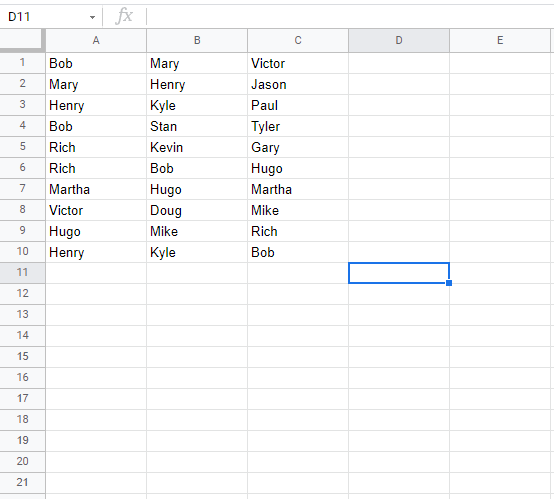
When we enter our conditional format rules, Apply to Range becomes A1:C10 and our custom formula becomes:
=COUNTIF($A$2:G,Indirect(Address(Row(),Column(),)))>1
This will highlight all duplicates across all three columns and all 10 rows, making it easy to spot data doppelgangers:
Dealing With Duplicates in Duplicates in Google Sheets
Can you highlight duplicates in Google Sheets? Absolutely. While the process takes more effort than some other spreadsheet solutions, it’s easy to replicate once you’ve done it once or twice, and once you’re comfortable with the process you can scale up to find duplicates across rows, columns, and even much larger data sets.

![]()